教育网站制作哪个好_站长工具源码_企业网站建设的重要性_江苏seo网络

用 ViT 做一个简单的图像分类任务

在 CIFAR-10 数据集上进行图像分类。通过 Hugging Face 的 transformers 库，加载一个预训练的 ViT 模型，并使用 PyTorch 进行微调。通过训练模型，评估测试集上的准确性，并可视化部分预测结果

可以将此方法应用到其他数据集或任务上，只需调整数据加载部分以及输出类别数

目录

1 创建环境并安装必要的库

2 导入依赖项

3 数据准备

4 加载 ViT 模型

5 训练模型 train.py

6 测试和评估 eval.py

7 可视化结果 plot.py

---

1 创建环境并安装必要的库

1. Anaconda 创建环境

conda create -n ViT python=3.8

2. 激活环境

conda activate ViT

3. 安装所需的库

pip install torch torchvision transformers matplotlib

2 导入依赖项

import torch
from torch import nn
from torchvision import datasets, transforms
from transformers import ViTForImageClassification, ViTFeatureExtractor
import matplotlib.pyplot as plt

3 数据准备

使用 CIFAR-10 数据集作为例子，该数据集包含10个类别的彩色图像。用以下代码加载和预处理数据集

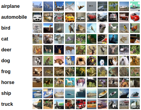
CIFAR-10 数据集由10个类别的60000张32x32彩色图像组成，每个类别有6000张图像。有50000个训练图像和10000个测试图像
数据集分为5个 training batches 和1个test batch，每个 batch 有10000张图像。test batch 包含从每个类别中随机选择的1000张图像。training batches 包含随机顺序的剩余图像，但某些 training batches 可能包含来自一个类的图像多于另一个类。在它们之间，training batches 包含来自每个类的5000张图像
以下是数据集中的类，以及每个类中的10张随机图像：

下载的是 python 版本，代码中会自动加载下载

# 定义图像预处理操作
transform = transforms.Compose([transforms.Resize((224, 224)),   # 调整图像大小为224x224，以适配ViTtransforms.ToTensor(),           # 转换图像为Tensortransforms.Normalize(mean=[0.485, 0.456, 0.406], std=[0.229, 0.224, 0.225])  # 标准化
])# 加载CIFAR-10数据集
train_dataset = datasets.CIFAR10(root='./data', train=True, download=True, transform=transform)
test_dataset = datasets.CIFAR10(root='./data', train=False, download=True, transform=transform)train_loader = torch.utils.data.DataLoader(train_dataset, batch_size=32, shuffle=True)
test_loader = torch.utils.data.DataLoader(test_dataset, batch_size=32, shuffle=False)# 检查标签的最小值和最大值
for images, labels in train_loader:print(labels.min(), labels.max())  # 确保标签值在0到9之间break

4 加载 ViT 模型

加载预训练的 ViT 模型有多种方法，可以参考之前的笔记文章——ViT 相关开源项目

此处使用 Hugging Face 的transformers库加载预训练的ViT模型

更具体而言，使用 ViTForImageClassification 模型，它已预训练并适合图像分类任务

# 加载预训练的ViT模型
model = ViTForImageClassification.from_pretrained('/home/yejiangchen/Desktop/Codes/ViT/config/')
# CIFAR-10有10个类别
model.classifier = nn.Linear(model.config.hidden_size, 10)  # 假设分类层的输出为10个类别
model = model.cuda()  # 如果有GPU，转移到GPU# 确保分类层已经正确初始化
print(model.classifier)  # 打印分类层以验证# 定义损失函数和优化器
criterion = nn.CrossEntropyLoss()
optimizer = torch.optim.Adam(model.parameters(), lr=1e-4)# 设置调试模式来帮助调试CUDA错误
os.environ['CUDA_LAUNCH_BLOCKING'] = "1"# 创建保存模型的文件夹
model_save_path = './models/'
if not os.path.exists(model_save_path):os.makedirs(model_save_path)

如果连接 Huggingface 超时，报错：

OSError: We couldn't connect to 'https://huggingface.co' to load this file, couldn't find it in the cached files and it looks like google/vit-base-patch16-224-in21k is not the path to a directory containing a file named config.json.
Checkout your internet connection or see how to run the library in offline mode at 'https://huggingface.co/docs/transformers/installation#offline-mode'.

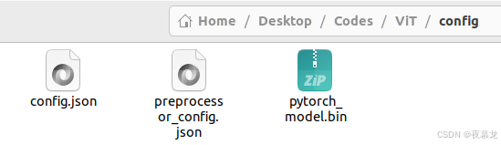
解决方法就是登上 huggingface，把 config.json、preprocessor_config.json、pytorch_model.bin下载到本地

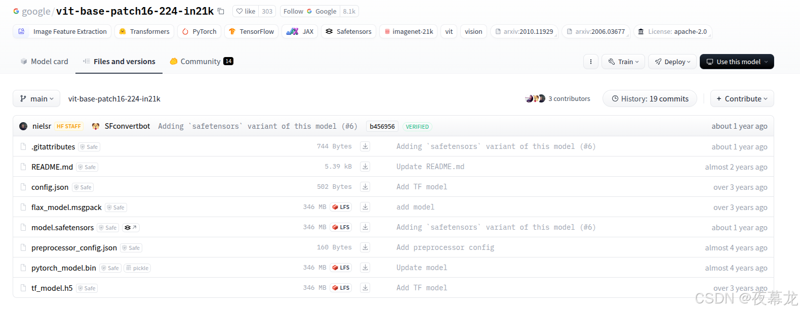
例如存在 config 文件夹中：

然后在调用模型时候采用如下本地加载的方式

model = ViTForImageClassification.from_pretrained('/home/yejiangchen/Desktop/Codes/ViT/config/')

5 训练模型 train.py

为了训练 ViT 模型，需要定义损失函数和优化器。此处使用交叉熵损失和 Adam 优化器

# 训练模型
epochs = 3  # 设置训练的epoch数量
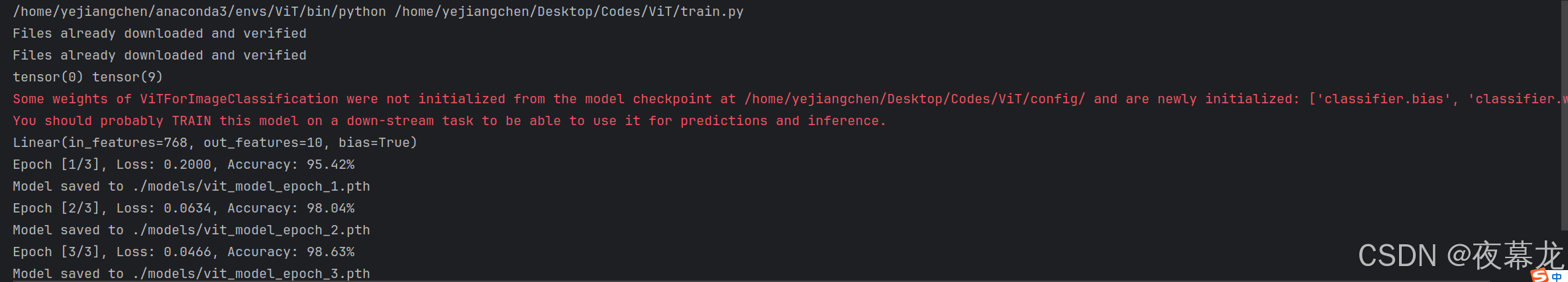
for epoch in range(epochs):model.train()running_loss = 0.0correct = 0total = 0for images, labels in train_loader:images, labels = images.cuda(), labels.cuda()# 前向传播outputs = model(images).logitsloss = criterion(outputs, labels)# 后向传播optimizer.zero_grad()loss.backward()optimizer.step()# 统计running_loss += loss.item()_, predicted = torch.max(outputs, 1)total += labels.size(0)correct += (predicted == labels).sum().item()# 打印每个epoch的损失和准确度print(f'Epoch [{epoch+1}/{epochs}], Loss: {running_loss/len(train_loader):.4f}, Accuracy: {100 * correct / total:.2f}%')# 每个epoch后保存模型model_filename = f'{model_save_path}vit_model_epoch_{epoch+1}.pth'torch.save(model.state_dict(), model_filename)print(f'Model saved to {model_filename}')

训练结果如下：

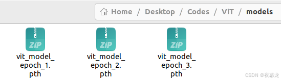
得到模型的权重参数文件：

6 测试和评估 eval.py

在测试阶段，需要加载训练好的模型，并在测试集上评估模型的性能

使用评估模式 model.eval() 来禁用训练过程中的某些操作（如 dropout）

import torch
import matplotlib.pyplot as plt
from torchvision import datasets, transforms
from transformers import ViTForImageClassification
from sklearn.metrics import confusion_matrix
import seaborn as sns
import numpy as np
import torch.nn as nn  # 这里导入 nn 模块# 定义图像预处理操作
transform = transforms.Compose([transforms.Resize((224, 224)),   # 调整图像大小为224x224，以适配ViTtransforms.ToTensor(),           # 转换图像为Tensortransforms.Normalize(mean=[0.485, 0.456, 0.406], std=[0.229, 0.224, 0.225])  # 标准化
])# 加载CIFAR-10测试集
test_dataset = datasets.CIFAR10(root='./data', train=False, download=True, transform=transform)
test_loader = torch.utils.data.DataLoader(test_dataset, batch_size=32, shuffle=False)# 加载训练后的模型
model = ViTForImageClassification.from_pretrained('/home/yejiangchen/Desktop/Codes/ViT/config/')
model.classifier = nn.Linear(model.config.hidden_size, 10)  # CIFAR-10有10个类别
model.load_state_dict(torch.load('./models/vit_model_epoch_3.pth'))  # 加载训练好的模型
model = model.cuda()  # 使用GPU# 将模型设置为评估模式
model.eval()# 记录预测结果和标签
all_labels = []
all_preds = []with torch.no_grad():  # 在评估阶段不计算梯度for images, labels in test_loader:images, labels = images.cuda(), labels.cuda()# 前向传播outputs = model(images).logits_, predicted = torch.max(outputs, 1)# 记录标签和预测all_labels.extend(labels.cpu().numpy())all_preds.extend(predicted.cpu().numpy())# 绘制混淆矩阵
cm = confusion_matrix(all_labels, all_preds)
plt.figure(figsize=(10, 8))
sns.heatmap(cm, annot=True, fmt='d', cmap='Blues', xticklabels=test_dataset.classes, yticklabels=test_dataset.classes)
plt.xlabel('Predicted')
plt.ylabel('True')
plt.title('Confusion Matrix')
plt.show()# 随机显示一些预测结果
import random
for _ in range(5):idx = random.randint(0, len(test_dataset) - 1)image, label = test_dataset[idx]image = image.unsqueeze(0).cuda()output = model(image).logits_, predicted = torch.max(output, 1)plt.imshow(image.squeeze().cpu().permute(1, 2, 0))plt.title(f'True: {test_dataset.classes[label]} | Predicted: {test_dataset.classes[predicted]}')plt.show()

运行结果如下：

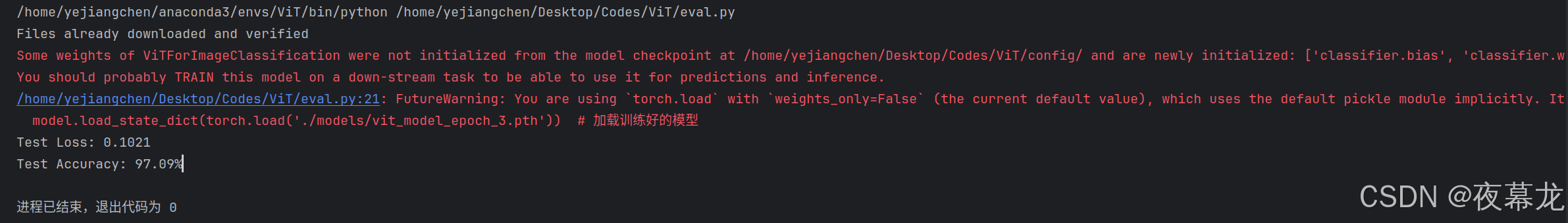
模型已经成功完成了评估，输出了测试集上的损失（Test Loss: 0.1021）和准确率（Test Accuracy: 97.09%）。这表明模型在测试集上的表现非常好，具有较高的准确率

测试损失（Test Loss）：表示模型在测试集上的损失函数值，通常损失越低表示模型越优秀

测试准确率（Test Accuracy）：模型在测试集上正确分类的样本占所有样本的比例，97.09% 表示模型能够正确分类绝大部分测试集样本

7 可视化结果 plot.py

为了更好地理解模型的性能，将测试结果可视化。通常绘制混淆矩阵和预测样本

• 混淆矩阵：使用 sklearn.metrics.confusion_matrix 生成混淆矩阵，并通过 seaborn 的 heatmap 绘制热图。混淆矩阵显示了真实标签与预测标签之间的关系，帮助了解哪些类别易混淆
• 预测样本：随机选择几张图像，并展示其真实标签与模型预测标签，以便直观评估模型性能

安装额外的库：

pip install scikit-learn
pip install seaborn

运行结果如下：

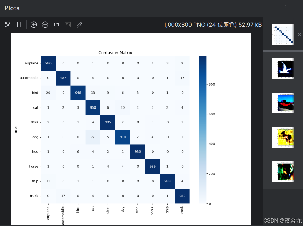
每行表示真实标签，每列表示模型的预测结果，矩阵中的数字显示了模型预测的数量

混淆矩阵分析：

• 对角线上的数值（如 airplane 类的986）表示模型正确预测的数量，数字越大，模型对该类别的预测越准确
• 非对角线上的数值表示误分类的情况。例如，bird 类被错误地预测为其他类别的次数。通过混淆矩阵，可以发现哪些类别之间容易混淆，进而进行优化

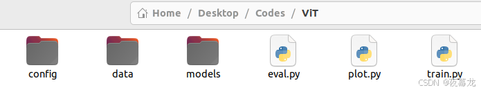
最后可以看到一个简单的项目的几个文件：