【人工智能学习之图像操作（四）】

图像金字塔

高斯金字塔

import cv2
img = cv2.imread(r"1.jpg")
for i in range(3):cv2.imshow(f"img{i}",img)img = cv2.pyrDown(img)
cv2.waitKey(0)

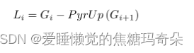
拉普拉斯金字塔

拉普拉斯金字塔由高斯金字塔计算得来

import cv2
img = cv2.imread(r"1.jpg")
img_down = cv2.pyrDown(img)
img_up = cv2.pyrUp(img_down)
img_new = cv2.subtract(img, img_up)
#为了更容易看清楚，做了个提高对比度的操作
img_new = cv2.convertScaleAbs(img_new, alpha=5, beta=0)
cv2.imshow("img_LP", img_new)
cv2.waitKey(0)

模板匹配

即使用模板匹配在一幅图像中查找目标

• 单对象匹配
• 多对象匹配
• cv2.TM_CCOEFF、 cv2.TM_CCOEFF_NORMED、cv2.TM_CCORR、cv2.TM_CCORR_NORMED、cv2.TM_SQDIFF、cv2.TM_SQDIFF_NORMED
  • 函数：cv2.matchTemplate()，cv2.minMaxLoc()
  • 注意：如果你使用的比较方法是 cv2.TM_SQDIFF和cv2.TM_SQDIFF_NORMED，最小值对应的位置才是匹配的区域。
  • 原理
    模板匹配是用来在一副大图中搜寻查找模版图像位置的方法。OpenCV 为我们提供了函数：cv2.matchTemplate()。和 2D 卷积一样，它也是用模板图像在输入图像（大图）上滑动，并在每一个位置对模板图像和与其对应的输入图像的子区域进行比较。OpenCV 提供了几种不同的比较方法（细节请看文档）。返回的结果是一个灰度图像，每一个像素值表示了此区域与模板的匹配程度。
    如果输入图像的大小是（WxH），模板的大小是（wxh），输出的结果的大小就是（W-w+1，H-h+1）。当你得到这幅图之后，就可以使用函数cv2.minMaxLoc() 来找到其中的最小值和最大值的位置了。第一个值为矩形左上角的点（位置），（w，h）为 moban 模板矩形的宽和高。这个矩形就是找到的模板区域了。

单对象匹配

import cv2
img = cv2.imread('1.jpg', 0)
template = cv2.imread('2.jpg', 0)
h, w = template.shape
res = cv2.matchTemplate(img, template, cv2.TM_CCOEFF)
min_val, max_val, min_loc, max_loc = cv2.minMaxLoc(res)
bottom_right = (max_loc[0] + w, max_loc[1] + h)
cv2.rectangle(img, max_loc, bottom_right, 255, 2)
cv2.imshow("img", img)
cv2.waitKey(0)

多对象匹配

import cv2
import numpy as np
img_rgb = cv2.imread('3.jpg')
img_gray = cv2.cvtColor(img_rgb, cv2.COLOR_BGR2GRAY)
template = cv2.imread('4.jpg', 0)
h, w = template.shape
res = cv2.matchTemplate(img_gray, template, cv2.TM_CCOEFF_NORMED)
loc = np.where(res >= 0.8)
for pt in zip(*loc[::-1]):
cv2.rectangle(img_rgb, pt, (pt[0] + w, pt[1] + h), (0, 0, 255), 2)
cv2.imshow('img', img_rgb)
cv2.waitKey(0)

无缝融合

我们可以利用金字塔对两种物体进行无缝对接

融合步骤

1. 读入两幅图像，苹果和橘子
2. 构建苹果和橘子的高斯金字塔（6 层）
3. 根据高斯金字塔计算拉普拉斯金字塔
4. 在拉普拉斯的每一层进行图像融合（苹果的左边与橘子的右边融合）
5. 根据融合后的图像金字塔重建原始图像。

import cv2
import numpy as np
A = cv2.imread('3.jpg')
B = cv2.imread('4.jpg')
# generate Gaussian pyramid for A
G = A.copy()
gpA = [G]
for i in range(6):
G = cv2.pyrDown(G)
gpA.append(G)
# generate Gaussian pyramid for B
G = B.copy()
gpB = [G]
for i in range(6):
G = cv2.pyrDown(G)
gpB.append(G)
# generate Laplacian Pyramid for A
lpA = [gpA[5]]
for i in range(5, 0, -1):
GE = cv2.pyrUp(gpA[i])
L = cv2.subtract(gpA[i - 1], GE)
lpA.append(L)
# generate Laplacian Pyramid for B
lpB = [gpB[5]]
for i in range(5, 0, -1):
GE = cv2.pyrUp(gpB[i])
L = cv2.subtract(gpB[i - 1], GE)
lpB.append(L)
# Now add left and right halves of images in each level
LS = []
for la, lb in zip(lpA, lpB):
rows, cols, dpt = la.shape
ls = np.hstack((la[:, 0:cols // 2], lb[:, cols // 2:]))
LS.append(ls)
# now reconstruct
ls_ = LS[0]
for i in range(1, 6):
ls_ = cv2.pyrUp(ls_)
ls_ = cv2.add(ls_, LS[i])
# image with direct connecting each half
real = np.hstack((A[:, :cols // 2], B[:, cols // 2:]))
cv2.imshow('Pyramid_blending.jpg', ls_)
cv2.imshow('Direct_blending.jpg', real)
cv2.waitKey(0)

Canny边缘提取算法

import cv2
img = cv2.imread("1.jpg", 0)
img = cv2.GaussianBlur(img, (3, 3), 0)
canny = cv2.Canny(img, 50, 150)
cv2.imshow('Canny', canny)
cv2.waitKey(0)

原理详解
步骤

• 彩色图像转换为灰度图像
• 高斯滤波，滤除噪声点
• 计算图像梯度，根据梯度计算边缘幅值与角度
• 非极大值抑制
• 双阈值边缘连接处理
• 二值化图像输出结果

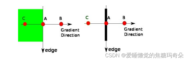
非极大值抑制
非极大值抑制是一种边缘稀疏技术，非极大值抑制的作用在于“瘦”边。对图像进行梯度计算后，仅仅基于梯度值提取的边缘仍然很模糊。而非极大值抑制则可以帮助将局部最大值之外的所有梯度值抑制为0

1. 将当前像素的梯度强度与沿正负梯度方向上的两个像素进行比较。
2. 如果当前像素的梯度强度与另外两个像素相比最大，则该像素点保留为边缘点，否则该像素点将被抑制。
   
   双阈值边缘连接处理
   这个阶段决定哪些边缘是边缘，哪些边缘不是边缘。为此，我们需要两个阈值，minVal和maxVal。强度梯度大于maxVal的边缘肯定是边缘，而minVal以下的边缘肯定是非边缘的，因此被丢弃. 两者之间的值要判断是否与真正的边界相连，相连就保留，不相连舍弃。

轮廓

轮廓查找与绘制

import cv2
img = cv2.imread('2.jpg')
imggray = cv2.cvtColor(img,cv2.COLOR_BGR2GRAY)
ret,thresh = cv2.threshold(imggray,127,255,0)
image, contours, hierarchy = cv2.findContours(thresh, cv2.RETR_TREE,cv2.CHAIN_APPROX_SIMPLE)
# image, contours, hierarchy = cv2.findContours(thresh, cv2.RETR_TREE,
cv2.CHAIN_APPROX_NONE)
img_contour= cv2.drawContours(img, contours, -1, (0, 255, 0), 3)
cv2.imshow("img_contour", img_contour)
cv2.waitKey(0)

面积，周长，重心

import cv2
img = cv2.imread('3.jpg', 0)
ret, thresh = cv2.threshold(img, 127, 255, 0)
_, contours, _ = cv2.findContours(thresh, cv2.RETR_TREE,
cv2.CHAIN_APPROX_SIMPLE)
M = cv2.moments(contours[0]) # 矩
cx, cy = int(M['m10'] / M['m00']), int(M['m01'] / M['m00'])
print("重心:", cx, cy)
area = cv2.contourArea(contours[0])
print("面积:", area)
perimeter = cv2.arcLength(contours[0], True)
print("周长:", perimeter)

轮廓近似

将轮廓形状近似到另外一种由更少点组成的轮廓形状，新轮廓的点的数目由我们设定的准确度来决
定。

import cv2
img = cv2.imread('3.jpg')
imggray = cv2.cvtColor(img,cv2.COLOR_BGR2GRAY)
ret,thresh = cv2.threshold(imggray,127,255,0)
_, contours, _ = cv2.findContours(thresh, cv2.RETR_TREE,
cv2.CHAIN_APPROX_SIMPLE)
epsilon = 60 #精度
approx = cv2.approxPolyDP(contours[0],epsilon,True)
img_contour= cv2.drawContours(img, [approx], -1, (0, 255, 0), 3)
cv2.imshow("img_contour", img_contour)
cv2.waitKey(0)

凸包与凸性检测

凸包与轮廓近似相似，但不同，虽然有些情况下它们给出的结果是一样的。
函数 cv2.convexHull() 可以用来检测一个曲线是否具有凸性缺陷，并能纠正缺陷。一般来说，凸
性曲线总是凸出来的，至少是平的。如果有地方凹进去了就被叫做凸性缺陷。
函数 cv2.isContourConvex() 可以可以用来检测一个曲线是不是凸的。它只能返回 True 或
False。

import cv2
img = cv2.imread('3.jpg')
imggray = cv2.cvtColor(img,cv2.COLOR_BGR2GRAY)
ret,thresh = cv2.threshold(imggray,127,255,0)
_, contours, _ = cv2.findContours(thresh, cv2.RETR_TREE,
cv2.CHAIN_APPROX_SIMPLE)
hull = cv2.convexHull(contours[0])
print(cv2.isContourConvex(contours[0]), cv2.isContourConvex(hull))
#False True
#说明轮廓曲线是非凸的，凸包曲线是凸的
img_contour= cv2.drawContours(img, [hull], -1, (0, 0, 255), 3)
cv2.imshow("img_contour", img_contour)
cv2.waitKey(0)

边界检测

• 边界矩形
• 最小矩形
• 最小外切圆

import cv2
import numpy as np
img = cv2.imread('4.jpg')
imggray = cv2.cvtColor(img, cv2.COLOR_BGR2GRAY)
ret, thresh = cv2.threshold(imggray, 127, 255, 0)
_, contours, _ = cv2.findContours(thresh, cv2.RETR_TREE,
cv2.CHAIN_APPROX_SIMPLE)
# 边界矩形
x, y, w, h = cv2.boundingRect(contours[0])
img_contour = cv2.rectangle(img, (x, y), (x + w, y + h), (0, 255, 0), 2)
# 最小矩形
rect = cv2.minAreaRect(contours[0])
box = cv2.boxPoints(rect)
box = np.int0(box)
img_contour = cv2.drawContours(img, [box], 0, (0, 0, 255), 2)
# 最小外切圆
(x, y), radius = cv2.minEnclosingCircle(contours[0])
center = (int(x), int(y))
radius = int(radius)
img_contour = cv2.circle(img, center, radius, (255, 0, 0), 2)
cv2.imshow("img_contour", img_contour)
cv2.waitKey(0)

import cv2
import numpy as np
img = cv2.imread('4.jpg')
imggray = cv2.cvtColor(img, cv2.COLOR_BGR2GRAY)
ret, thresh = cv2.threshold(imggray, 127, 255, 0)
_, contours, _ = cv2.findContours(thresh, cv2.RETR_TREE,
cv2.CHAIN_APPROX_SIMPLE)
# 椭圆拟合
ellipse = cv2.fitEllipse(contours[0])
cv2.ellipse(img, ellipse, (255, 0, 0), 2)
# 直线拟合
h, w, _ = img.shape
[vx, vy, x, y] = cv2.fitLine(contours[0], cv2.DIST_L2, 0, 0.01, 0.01)
lefty = int((-x * vy / vx) + y)
righty = int(((w - x) * vy / vx) + y)
cv2.line(img, (w - 1, righty), (0, lefty), (0, 0, 255), 2)
cv2.imshow("img_contour", img)
cv2.waitKey(0)

轮廓性质

• 边界矩形的宽高比

x,y,w,h = cv2.boundingRect(cnt)
aspect_ratio = float(w)/h

• 轮廓面积与边界矩形面积的比

area = cv2.contourArea(cnt)
x,y,w,h = cv2.boundingRect(cnt)
rect_area = w*h
extent = float(area)/rect_area

• 轮廓面积与凸包面积的比

area = cv2.contourArea(cnt)
hull = cv2.convexHull(cnt)
hull_area = cv2.contourArea(hull)
solidity = float(area)/hull_area

• 与轮廓面积相等的圆形的直径

area = cv2.contourArea(cnt)
equi_diameter = np.sqrt(4*area/np.pi)

• 对象的方向
  下面的方法还会返回长轴和短轴的长度

(x,y),(MA,ma),angle = cv2.fitEllipse(cnt)