目录
- 一、历史
- 二、精髓思想
- 三、案例与代码实现
一、历史
- 问:谁在什么时候提出模拟退火?
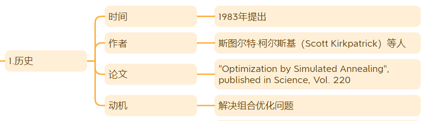
- 答:模拟退火算法(Simulated Annealing,SA)是由斯图尔特·柯尔斯基(Scott Kirkpatrick) 等人在 1983年 提出的。
- 论文:“Optimization by Simulated Annealing”, published in Science, Vol. 220
- 动机:解决组合优化问题
二、精髓思想
- 精髓就两字:退火!
- 解释:字面意思就是模拟打铁的退火过程,刚开始打铁吧温度比较高,铁烧的红红的容易打出各种形状,随着时间变长,温度逐渐冷却下来,铁更硬了,形状大方向基本确定。
不禁感叹,以前的物理学家、数学家灵感来源都是自然现象!

总结下来其实就3个step:
- 拿一块铁过来淬火
- 打一次看看如何
- 给我打到定型
三、案例与代码实现
-
题干:
6艘船靠3个港口,已知达到时间arrival和卸货时长handling,求最优停靠方案,即等待时长最短。 -
数据:
ships = {'S1': {'arrival': 0.1, 'handling': 4},'S2': {'arrival': 2.1, 'handling': 3},'S3': {'arrival': 4.2, 'handling': 2},'S4': {'arrival': 6.3, 'handling': 3},'S5': {'arrival': 5.5, 'handling': 2},'S6': {'arrival': 3.9, 'handling': 4},'S7': {'arrival': 3.7, 'handling': 4},'S8': {'arrival': 3.4, 'handling': 4},
}
- 实现:
step1:拿一块铁过来淬火
# 随机初始化一块铁(船舶调度顺序)
initial_order = list(ships.keys()) # 船舶原始顺序['S1', 'S2', 'S3', 'S4', 'S5', 'S6', 'S7', 'S8']
random.shuffle(initial_order)	#	打乱顺序 ,可能是['S2', 'S7', 'S6', 'S5', 'S1', 'S3', 'S4', 'S8']
- step2:打一次看看如何
首先,先评价一下原始模样如何?用等待时间作为衡量,如下:
current_cost = evaluate(current)
NUM_BERTHS = 3  # 泊位数量
# 评价函数:计算某个调度顺序的总等待时间
def evaluate(order):berth_times = [0] * NUM_BERTHStotal_wait = 0for ship_id in order:arrival = ships[ship_id]['arrival']handling = ships[ship_id]['handling']# 找到最早可用泊位berth_index = min(range(NUM_BERTHS), key=lambda i: max(arrival, berth_times[i]))# start_time = 开始卸货时间 = max(到达时间, 泊位可用时间)。# 解释:要卸货的话,船先到达了没有泊位可用也得等,反之,有空泊位了船还没到也得等。start_time = max(arrival, berth_times[berth_index])wait_time = start_time - arrivaltotal_wait += wait_timeberth_times[berth_index] = start_time + handlingreturn total_wait
然后,开始下锤子了(称之为扰动)
# 生成邻域解(随机交换两艘船顺序)
def neighbor(order):new_order = order.copy()i, j = random.sample(range(len(order)), 2)new_order[i], new_order[j] = new_order[j], new_order[i]return new_order
紧接着,评估下现在模样和上一次区别,如下:
new = neighbor(current)
new_cost = evaluate(new)
delta = new_cost - current_cost	# 扰动之后的区别
最后,做决定是接着现在模样往下继续打,还是恢复回原来模样
# 情况1:delta < 0 说明等待时间变短了呀,打铁打得更好了,欣然接受。
# 情况2:delta >= 0 说明等待时间变长了,糟糕打偏了,不过没关系,这是艺术啊!不完美也是一种美!看心情决定~
# 于是有了 random.random() < math.exp(-delta / T)这一项
# 解释:random.random()就是一个随机值(类比于当时心情),值域范围[0.0, 1.0)
# math.exp(-delta / T)和delta、T有关系,这么来看吧,假设现在超级无敌高温,那么-delta / T趋于0,那么math.exp(-delta / T)趋于1,说明有很大概率接受比较差的解。假设现在温度快降到0了,那么-delta / T趋于负无穷,那么math.exp(-delta / T)趋于0,说明有极小概率接受比较差的解。
if delta < 0 or random.random() < math.exp(-delta / T):current = newcurrent_cost = new_cost
- step3:给我打到定型
循环的过程,就是往复step2的过程,持续下去直到定型,如下:
# 模拟退火主过程
# 初始顺序:initial_order, 温度:T=100.0, 冷却率:cooling_rate=0.95, 最低温度:T_min=1e-3
def simulated_annealing(initial_order, T=100.0, cooling_rate=0.95, T_min=1e-3):current = initial_ordercurrent_cost = evaluate(current)best = currentbest_cost = current_costwhile T > T_min:for _ in range(100):  # 每个温度尝试多次扰动new = neighbor(current)new_cost = evaluate(new)delta = new_cost - current_costif delta < 0 or random.random() < math.exp(-delta / T):current = newcurrent_cost = new_costif current_cost < best_cost:best = currentbest_cost = current_costT *= cooling_rate  # 降温return best, best_cost